Why Neural Networks Fail on Constraints and why Lagrangian Geometry works better

Neural networks are extremely good at learning patterns, but they struggle when the problem demands obedience rather than approximation. In particular, they often fail when outputs must satisfy strict rules, conservation laws, geometric consistency, physical constraints and sometimes even logical structure.

This failure is not a matter of insufficient data or model size. It is geometric. In this article, I argue that hard-constraint problems define lower-dimensional geometric objects inside high-dimensional spaces, and that standard neural network training does not naturally respect these objects. By viewing constraints through the lens of geometry, I believe we can gain a clearer understanding on how to tackle these problems.

What is a constraint and what should classify as one?

A constraint is simply a rule that says that not everything is allowed. You can think of it as a fence that blocks a wall. Operating inside the wall is very permissible, but outside of it is invalid. So a constraint limits what is required as input or output depending on the nature.

Formally, we define the following.

Let $\mathcal{X}$ be the input space and $\mathcal{Y}$ be the output space.

A model (neural network) is defined as:

$$f_\theta : \mathcal{X} \rightarrow \mathcal{Y}$$

A constraint is a condition that restricts the set of admissible outputs.

Formally, a constraint is a function:

$$c : \mathcal{Y} \rightarrow \mathbb{R}^k$$

with feasibility conditions such as:

Equality constraint:

$$c(y) = 0$$

Inequality constraint:

$$c(y) \le 0$$

These constraints define the feasible set:

$$\mathcal{Y}_{\text{feasible}} := \left\{y \in \mathcal{Y} \;\middle|\; c(y) = 0 \;\text{and/or}\; c(y) \le 0 \right\}$$

Any output is considered invalid if:

$$y \notin \mathcal{Y}_{\text{feasible}}$$

What should classify as a constraint?

Basically, anything that restricts a space can be classified as a constraint. But this raises an important question: how do we identify a constraint mathematically?

It turns out that identifying constraints is much easier than it first appears. The key idea is simple: a constraint is anything that removes degrees of freedom from a space. In other words, it shrinks the set of allowable configurations.

Mathematically, this happens whenever we impose a condition that restricts a space $\mathcal{Y} \subseteq \mathbb{R}^n$ to a smaller subset $\mathcal{Y}_{\text{feasible}} \subset \mathcal{Y}.$ This restriction may take the form of equations, inequalities, or structural rules, but the effect is always the same: not every point in the original space is allowed.

Examples of constraints would include algebraic manifolds and normalization conditions. My argument is that the root cause is geometric: standard neural training optimizes in parameter space, while constraints live on manifolds in output space.

Modern neural networks are universal function approximators, yet universality does not imply constraint satisfaction. It actually turns out that models trained with standard empirical risk minimization frequently violates a number of constraints like physical conservation laws, Normalization constraints and even algebraic invariant.

One of the ways that is used to solve this is by adding a penalty term to the loss function. Surprisingly, we can only get something good using excessively large penalty coefficients.

Learning with Hard Constraints.

Let us take a look at a classical problem involving learning with hard constraints.

Let a neural network be defined as

$$y = f_\theta(x),$$

with parameters $\theta \in \mathbb{R}^d$ Suppose the output must satisfy a hard constraint $g(y) = 0,$

where

$$g: \mathbb{R}^k \to \mathbb{R}^m.$$

The learning objective becomes a constrained optimization problem:

$$\min_\theta \mathcal{L}_{\text{data}}(f_\theta(x)) \quad \text{subject to} \quad g(f_\theta(x)) = 0.$$

The feasible outputs lie on a manifold

$$\mathcal{M} = \{ y \mid g(y) = 0 \}$$

What is a manifold?

A manifold is a curved surface that looks flat when zoomed in on it. Think of the earth. From an outer viewpoint, the earth is spherical and curved; but inside of the sphere appears to be locally flat. We say that a manifold is thus a curved surface that is locally Euclidean. More subtly, a manifold appears whenever constraints reduce freedom without destroying smoothness.

Informal definition

An n-dimensional manifold is a space that, around every point, looks like ordinary $\mathbb{R}^n.$

Formally:

A topological space $\mathcal{M}$ is an n-dimensional (smooth) manifold if for every point $p \in \mathcal{M}$, there exists:

1. An open neighborhood $U \subset \mathcal{M}$ containing p

2. A map (called a chart)

$$\varphi: U \rightarrow \mathbb{R}^n$$

such that:

• $\varphi$ is bijective
• $\varphi$ is continuous
• $\varphi^{-1}$ is continuous

This means:

$$U \approx \mathbb{R}^n$$

Smooth manifolds

A manifold is smooth if whenever two charts of the manifold overlap, their transition map is smooth.

Let

$$\varphi_i: U_i \rightarrow \mathbb{R}^n, \quad \varphi_j: U_j \rightarrow \mathbb{R}^n$$

Then the map

$$\varphi_j \circ \varphi_i^{-1} : \varphi_i(U_i \cap U_j) \rightarrow \varphi_j(U_i \cap U_j)$$

must be infinitely differentiable $C^\infty$

Embedded (constraint-defined) manifolds

Now let us define manifolds in the sense of constraints, which is the essence of this article. Before I put out the mathematics, let us try to get the idea behind constraint-defined manifolds.

Imagine you've got a huge playground. You're allowed to move around anywhere on the playground unrestricted. Now assume that a teacher marks a tape around the playground. The tape twists and turns and creates varying paths on the playground. The teacher says you're not allowed to move beyond the paths marked by the tape. This means that you're now constrained by the tape.

The tape is the rule that you must follow (the constraint) Despite shifting and turning, each path on the tape feels locally flat. The track created by the tape is the manifold and it lives inside the playground. Now we can formally define the constraint-defined manifold.

Let:

$$c : \mathbb{R}^m \rightarrow \mathbb{R}^k$$

Define:

$$\mathcal{M} = \{ y \in \mathbb{R}^m \mid c(y) = 0 \}$$

If:

• c is smooth
• The Jacobian $\nabla c(y)$ has full rank k on $\mathcal{M}$

Then $\mathcal{M}$ is a smooth manifold of dimension $m - k$

The penalty Method

Let us go back a bit to our playground analogy. Now put a baby in the playground and ask him to follow these rules. Definitely the baby has no idea what the rule is and is used to moving around freely in the open playground space. To constrain the baby, you introduce murky sand or muddy water on the other parts outside the tape. The is still allowed to move freely, but when he gets outside the tape, he is stuck in muddy water and requires a lot more energy to push through. Gradually after multiple punishment, the baby learns to stay within the taped path. This is exactly what the penalty method does. To constrain the neural network (NN), we introduce a penalty term. The penalty term relaxes the constraint to give meaningful outcomes.

$$\mathcal{L}_{\text{pen}}(\theta) = \mathcal{L}_{\text{data}}(\theta) + \lambda \| g(f_\theta(x)) \|^2$$

As $\lambda \to \infty$, optimization theory suggests convergence to the constrained solution. However, neural networks slightly violate these assumptions under which this guarantee holds.

Now in practice, using very large $\lambda$ may work but at what cost? Well, empirically, increasing $\lambda$ often causes gradient domination by the penalty term, optimization instability and poor convergence to feasible solutions.

"Penalty methods can approximate the constraint by making $\lambda$ large, achieving violations on the order of $10^{-3}$ to $10^{-4}$. However, this comes at severe costs: gradients become unstable with spikes exceeding $10^3$, training slows dramatically, and exact constraint satisfaction (violation = 0) is never achieved. As $\lambda \to \infty$, the optimization problem becomes ill-conditioned. For applications requiring hard constraints satisfaction is insufficient."

In summary, penalty methods apply forces orthogonal to the manifold but do not guarantee tangential consistency. As a result, the optimizer oscillates near the manifold without converging to it.

The ideas above are implemented in a Colab notebook, where I compare penalty-based training against a Lagrangian formulation on a constrained toy problem. The code is intentionally separated to keep the focus here on geometry and intuition. View the Colab notebook

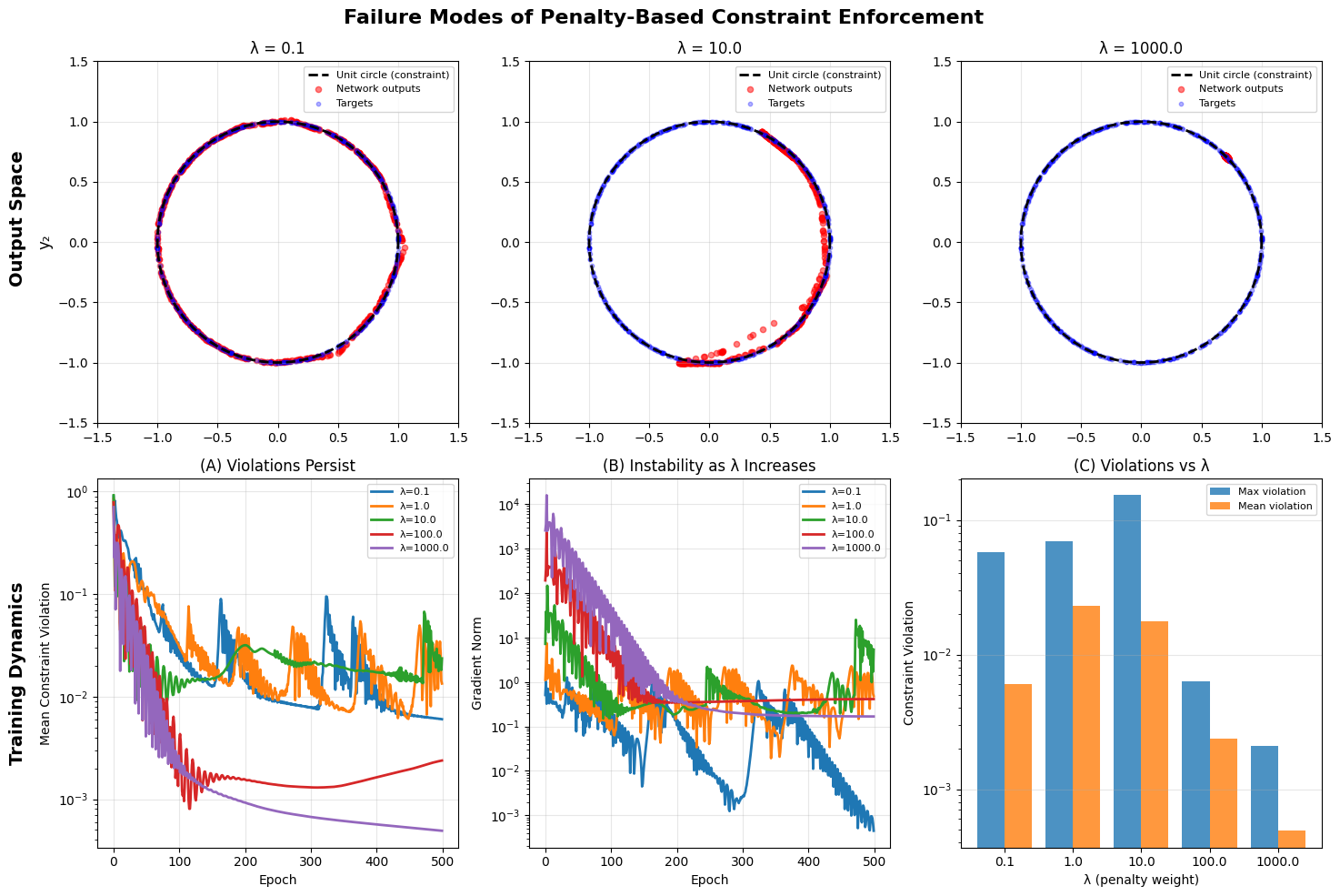Figure 1: The constraint manifold in output space

The Lagrangian

The penalty method encourages a neural network to stay close to the constraint manifold by punishing violations. However, this approach treats constraints as soft preferences. To enforce constraints more structurally, we introduce the Lagrangian formulation.

Suppose we want to minimize an objective function $\ell(y)$ subject to a constraint $c(y) = 0$. Instead of optimizing under an explicit restriction, we combine the objective and the constraint into a single function called the Lagrangian.

Formally, the Lagrangian is defined as:

$$\mathcal{L}(y, \lambda) = \ell(y) + \lambda \, c(y)$$

Here:

• y represents the model output or decision variable
• $c(y) = 0$ is the constraint
• $\lambda$ is the Lagrange multiplier, which controls how strongly the constraint is enforced

Intuitively, the Lagrange multiplier acts like a learnable force that pushes solutions back onto the constraint manifold whenever they drift away.

Lagrangian Formulation

The correct constrained objective is given by the Lagrangian:

$$\mathcal{L}(\theta, \lambda) = \mathcal{L}_{\text{data}}(\theta) + \lambda^T g(f_\theta(x))$$

Unlike penalty methods, the Lagrangian introduces dual variables that adaptively enforce constraints.

The update then becomes

$$\theta_{t+1} = \theta_t - \eta_\theta \nabla_\theta \mathcal{L},$$ $$\lambda_{t+1} = \lambda_t + \eta_\lambda g(y)$$

This defines a primal-dual dynamical system

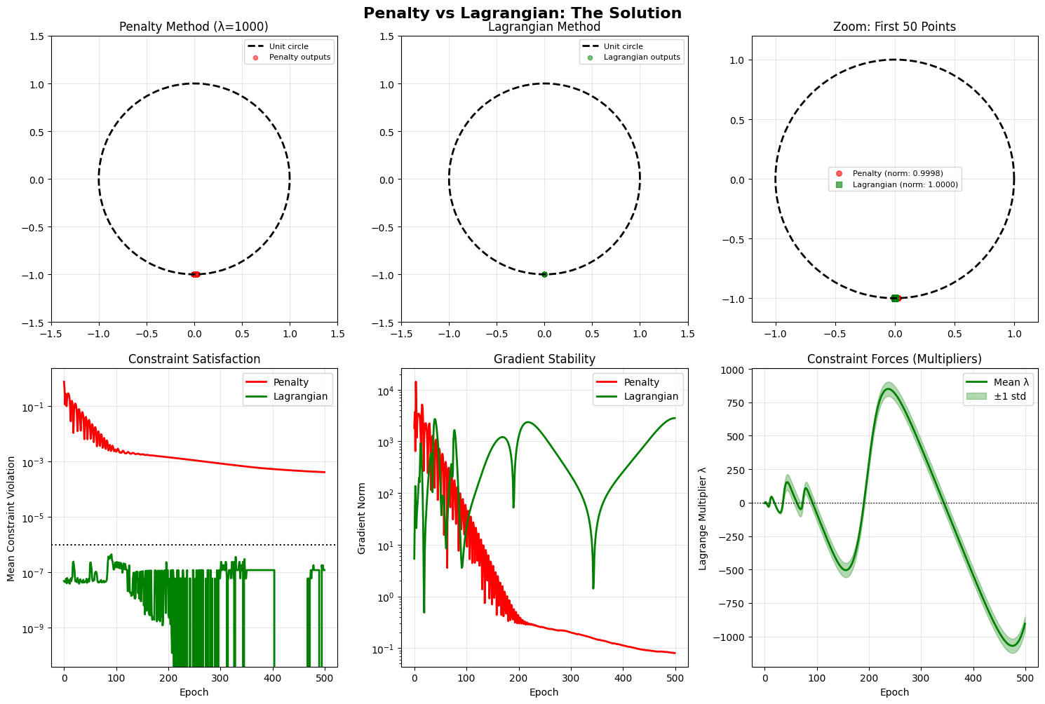
Why this matters for neural networks?

Neural networks naturally operate in unconstrained spaces. The Lagrangian formulation provides a principled way to introduce constraints without collapsing optimization stability, allowing gradients to respect the geometry of the feasible manifold.

To see the effect of the lagrangian and how the results differ in comparison to the penalty method, you can take a look at the colab code attached below.

Conclusion

Hard constraints are not just additional loss terms or penalties to be tuned; they define geometry.

When a task demands exact satisfaction of constraints, the correct outputs live on a manifold - a thin, structured subset of the output space. Standard neural networks, trained with unconstrained optimization, have no inherent reason to remain on this manifold. They wander near it, approximate it, and often violate it.

Penalty methods attempt to push solutions toward feasibility, while Lagrangian formulations explicitly encode the geometry of the constraint surface. Both approaches acknowledge a fundamental truth: constrained learning is not just about minimizing error, but about respecting structure.

Understanding this distinction reframes the problem. Neural networks do not fail because they are weak function approximators, but because they are trained in spaces larger than the problem allows.

Once we see constraints as geometry, the path forward becomes clearer